[ML]All about Optimization

Optimization is a fundamental component of machine learning. In the process of training models using gradient descent, the objective is to iteratively minimize the loss function by adjusting the model’s parameters in the direction of the negative gradient. However, there are instances where the gradient descent algorithm converges to a point where further reduction in the loss becomes infeasible, often due to encountering a local minimum or saddle point.

Critical Point

A critical point refers to a point where the gradient is zero, which may temporarily halt the loss reduction process during gradient descent. There are three types of critical points: local minima, local maxima, and saddle points.

When a model reaches a local minimum or maximum, gradient descent effectively terminates as further improvement in loss is not possible. However, saddle points behave differently. Although the gradient is zero at a saddle point, there may still exist directions in which the loss can decrease. The task then becomes identifying those directions to escape the saddle point.

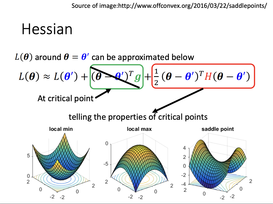
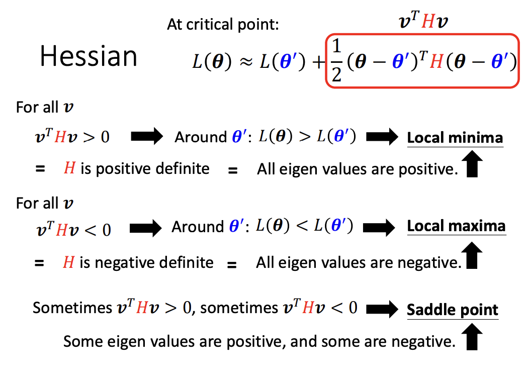
To classify a critical point, the Hessian matrix is used:

• If the Hessian matrix is positive definite (all eigenvalues are positive), the point is a local minimum.
• If the Hessian matrix is negative definite (all eigenvalues are negative), the point is a local maximum.
• If the Hessian matrix has both positive and negative eigenvalues, the point is classified as a saddle point.

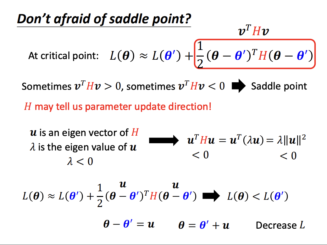
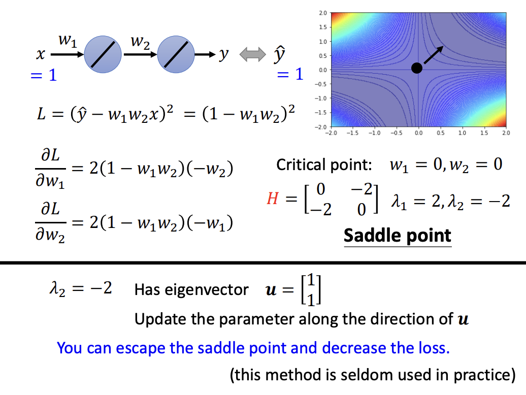
The Hessian matrix not only helps identify saddle points but also provides a way to determine the direction in which to move. By following the direction of an eigenvector corresponding to a negative eigenvalue, we can escape the saddle point and continue the optimization process.

Batch

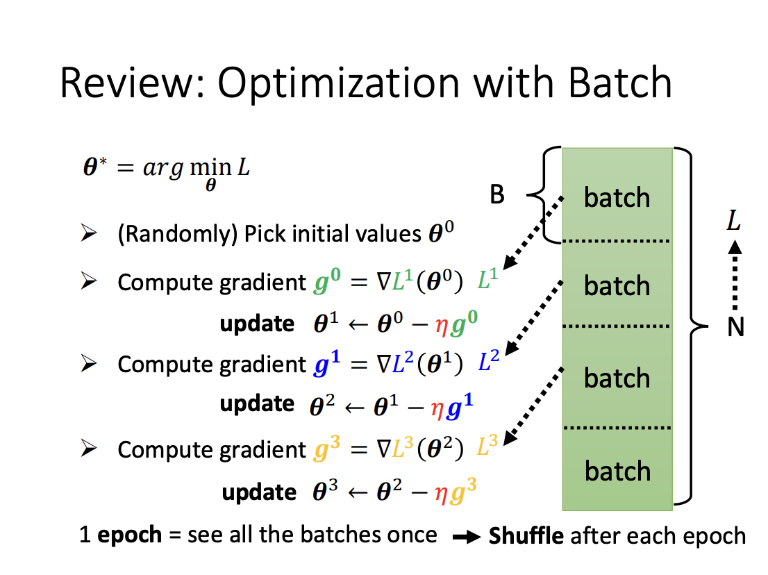
In model training, data is processed in batches, where a subset of the entire dataset is used for each training iteration. Once all batches have been processed, the full pass through the dataset is referred to as an epoch. Before each epoch, the data is randomly shuffled and then divided into batches, this process is known as shuffling.

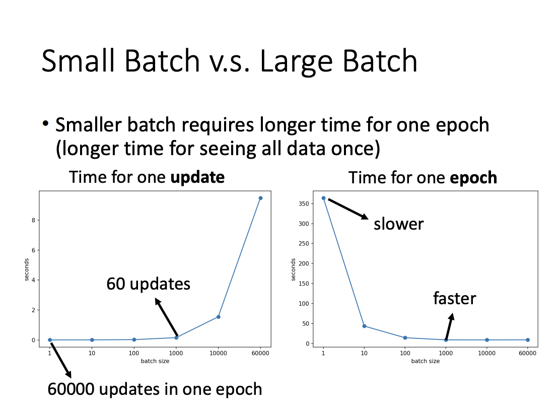
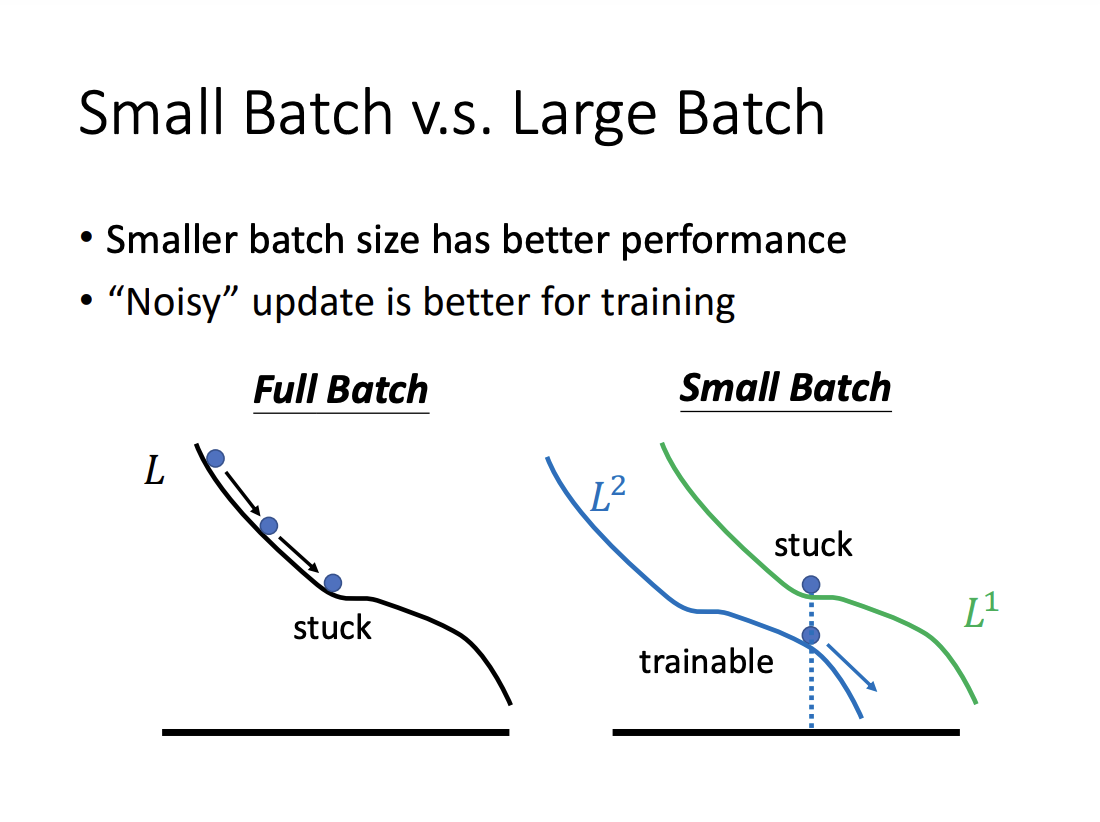
Batch size is a hyperparameter that needs to be determined. While it might seem intuitive that larger batch sizes would result in faster training, smaller batch sizes are often preferred, especially when using parallel computing. Although larger batches can reduce the number of updates per epoch, smaller batches typically allow for faster computations due to more efficient memory usage and hardware parallelism. Furthermore, smaller batch sizes introduce a higher level of noise in gradient updates, which has been shown to enhance generalization performance.

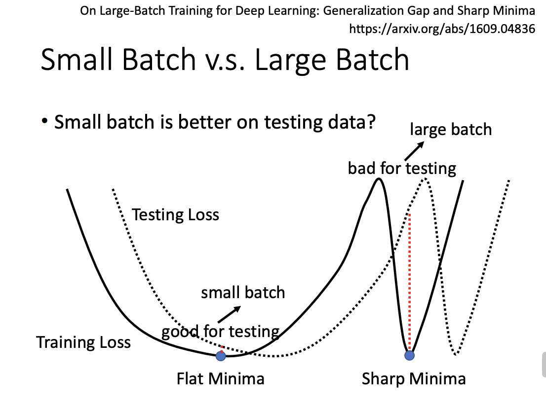
This noise in the updates is believed to help models converge to flat minima rather than sharp minima. Flat minima are associated with better generalization and robustness, while sharp minima may lead to poorer performance on unseen data.

Momentum

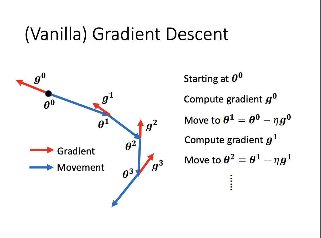
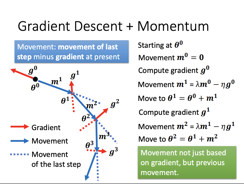
Vanilla Gradient Descent solely considers the current gradient direction when updating model parameters. In contrast, Momentum incorporates information from the previous update step by maintaining a velocity vector, which is a moving average of past gradients. This allows the optimizer to build inertia in the direction of consistent gradients, helping the model move more smoothly through the optimization landscape.

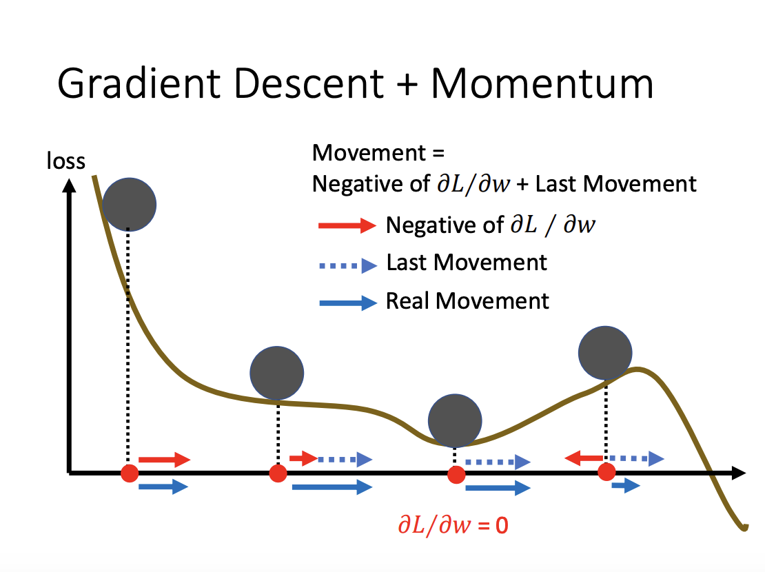
Momentum is particularly useful in escaping critical points such as saddle points, as it enables the optimizer to carry forward some velocity from previous updates, preventing it from getting stuck in areas where the gradient is close to zero.

Adaptive Learning Rate

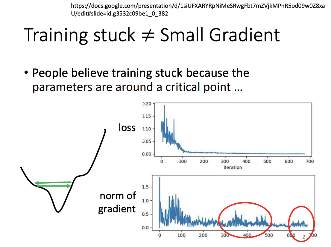
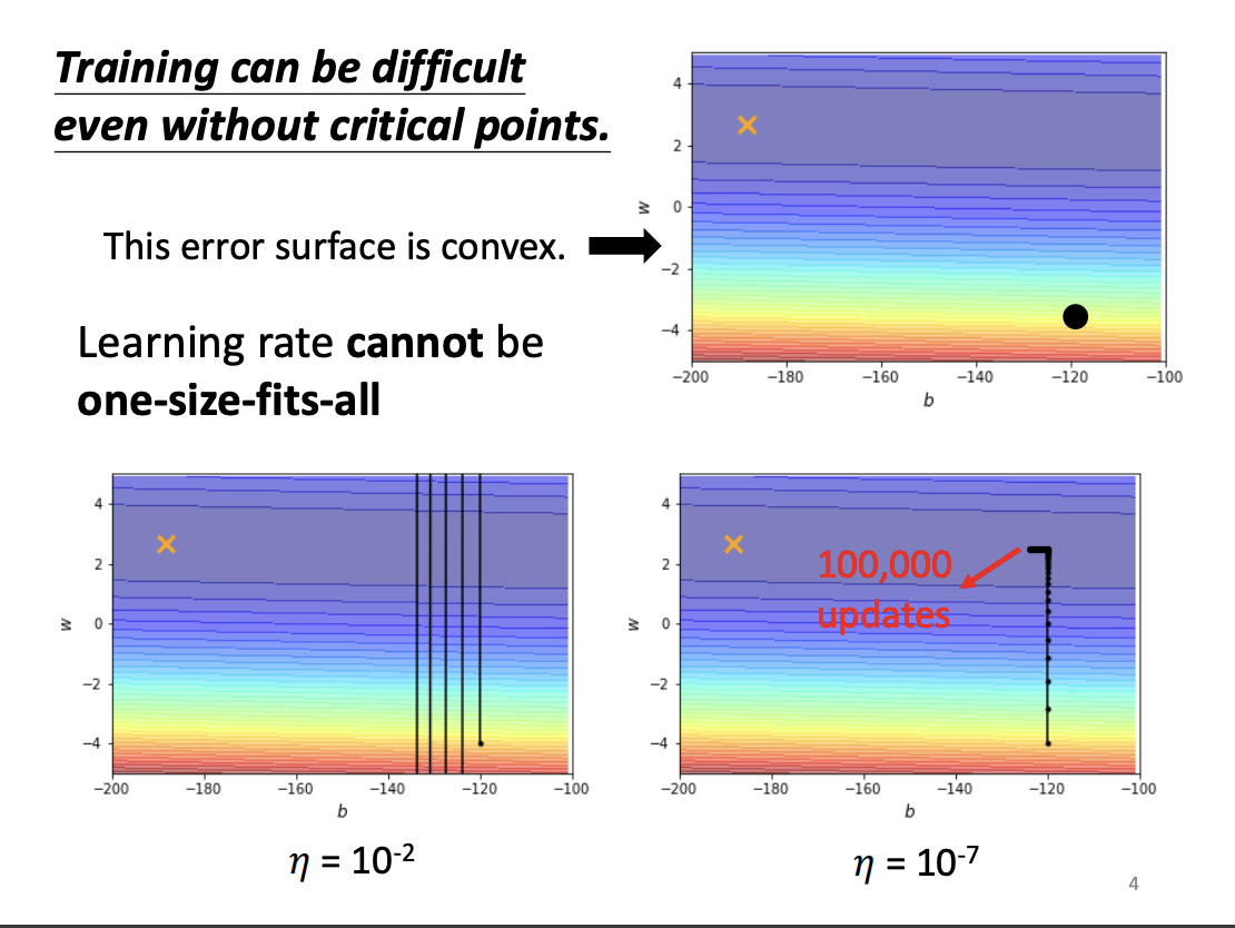
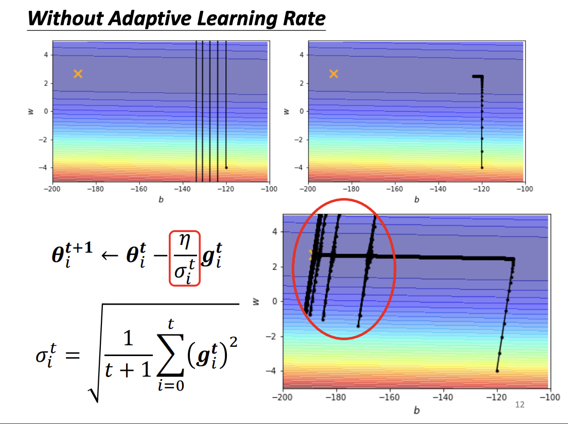
While critical points can impede training, they are relatively rare in practice. More commonly, training can stagnate when gradients become too large. To address this, it’s important to not only consider the direction of updates but also the size of the steps, which is determined by the learning rate.

Both excessively small and large learning rates can struggle to handle basic optimization challenges, such as traversing convex error surfaces. To mitigate this, adaptive learning rates are employed.

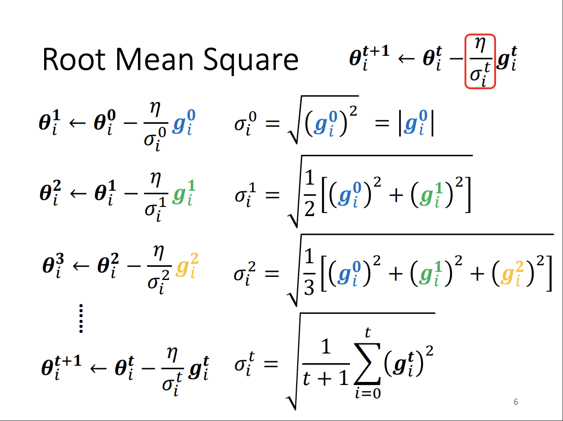
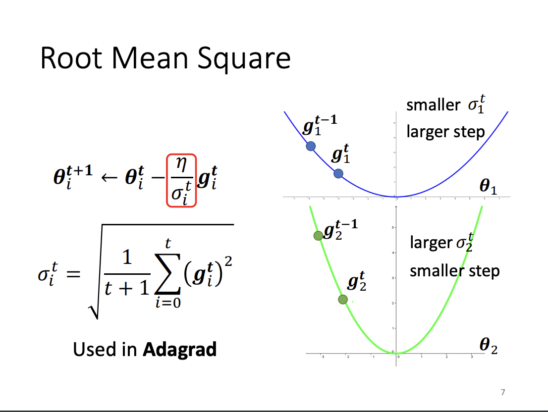
One widely used method for adaptive learning rates is Adagrad. In Adagrad, the learning rate is adjusted based on the magnitude of past gradient updates: small gradients receive a larger learning rate, while large gradients are assigned a smaller one. This ensures that the learning process is more stable across different scales of gradient changes.

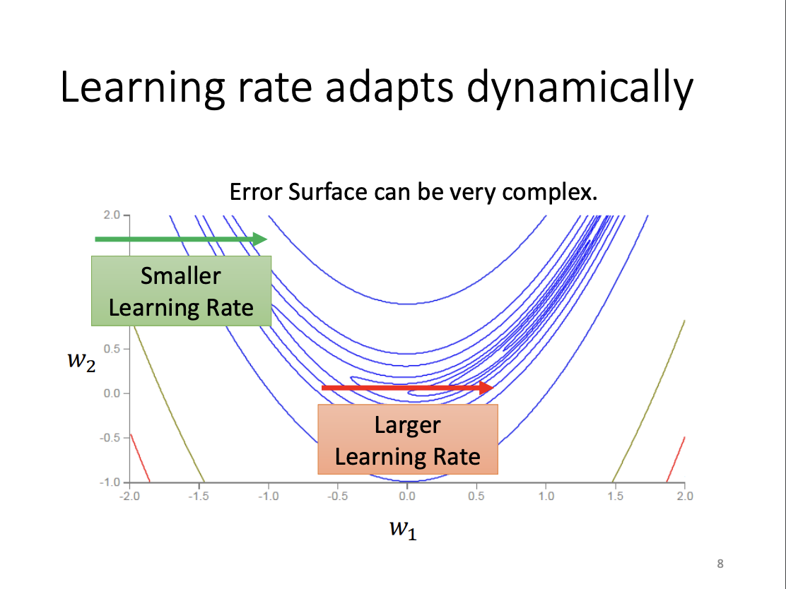
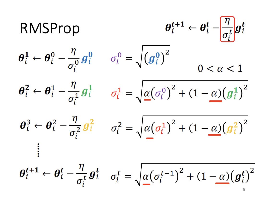
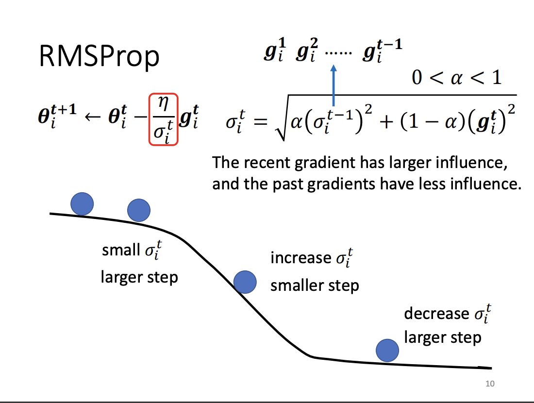
However, Adagrad is less effective in scenarios where gradients fluctuate between large and small values. To better handle such dynamic situations, RMSProp was introduced. Unlike Adagrad, RMSProp applies an exponential moving average to recent gradients, allowing the learning rate to adjust more responsively over time. The key difference is that RMSProp gives more weight to recent steps, rather than equally weighting all past steps as Adagrad does.

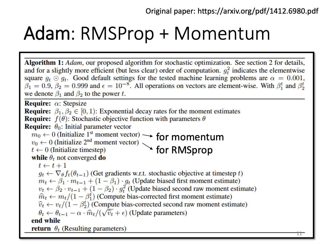
Adam (Adaptive Moment Estimation) combines the benefits of both RMSProp and Momentum, making it one of the most widely used optimization algorithms in modern machine learning.

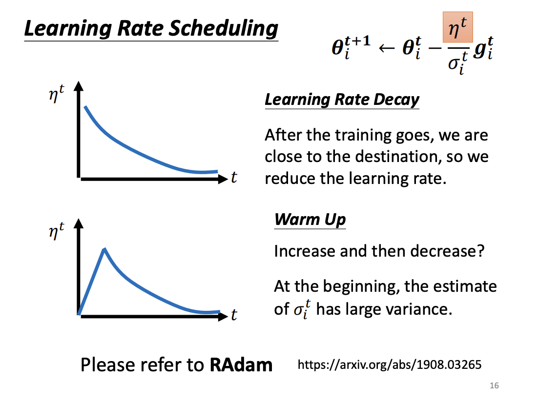
Learning Rate Scheduling

While methods like Adagrad adjust the learning rate based on gradient magnitudes, they can lead to issues such as the accumulation of small gradient updates over time, causing inefficiencies. To counteract this, learning rate scheduling is used to dynamically adjust the learning rate throughout the training process. Common strategies include learning rate decay, where the learning rate decreases over time, and warm-up, where the learning rate starts small and gradually increases before decaying. These techniques help the model avoid sharp oscillations and ensure smoother convergence.

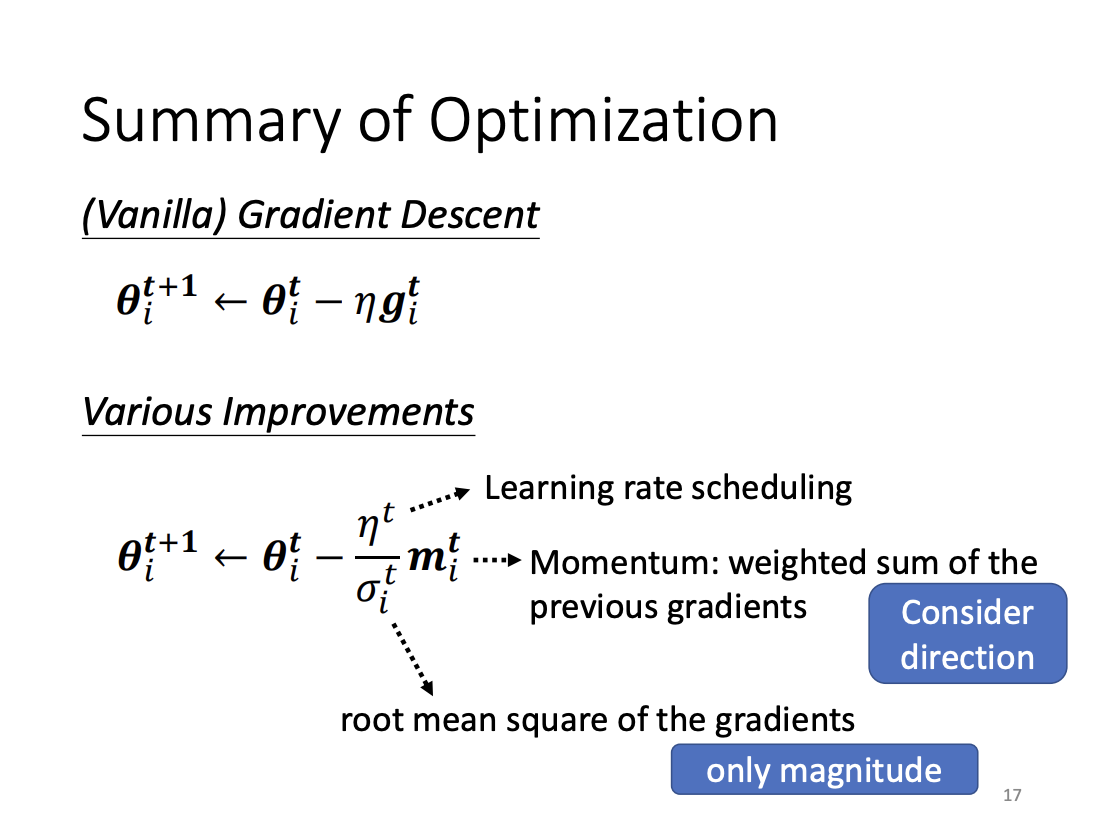
Interim Summary

To optimize gradient descent, we introduce Momentum to consider the direction of gradient changes by using a weighted sum of previous gradients. We also introduce Adagrad and RMSProp to adapt the learning rate based on the magnitude of past gradients. Finally, learning rate scheduling techniques like learning rate decay and warm-up help dynamically adjust the learning rate to maintain efficient training throughout the process.

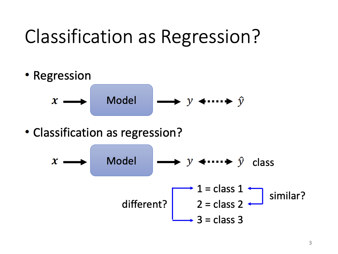
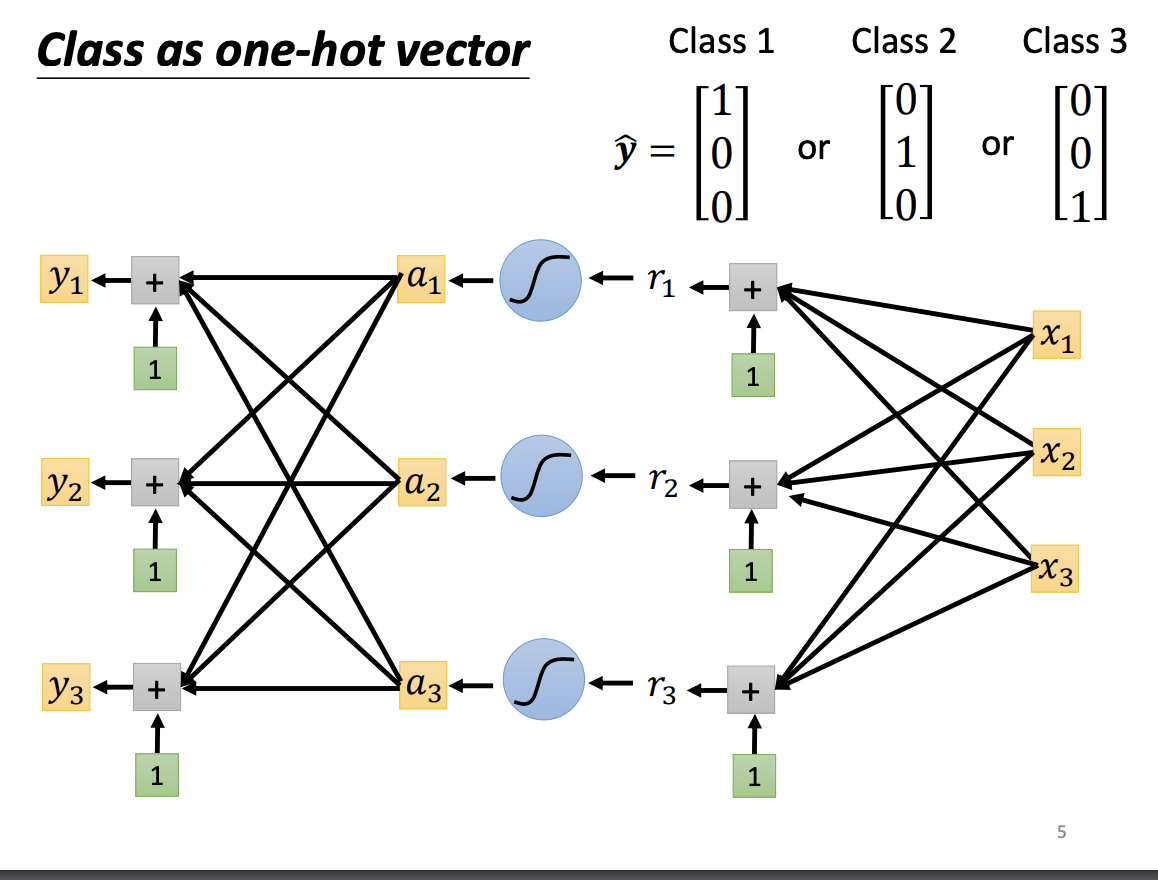
Classification

Regression and classification are two primary tasks in machine learning. The key distinction between them is that regression predicts a continuous value, while classification assigns an input to a discrete class. To represent these class types, a one-hot vector is commonly used, ensuring that each class is equidistant from the others in the vector space.

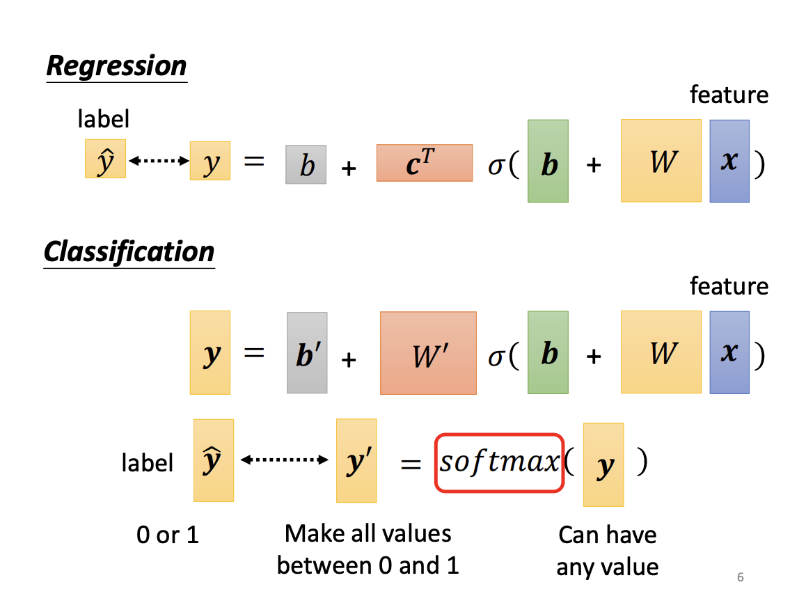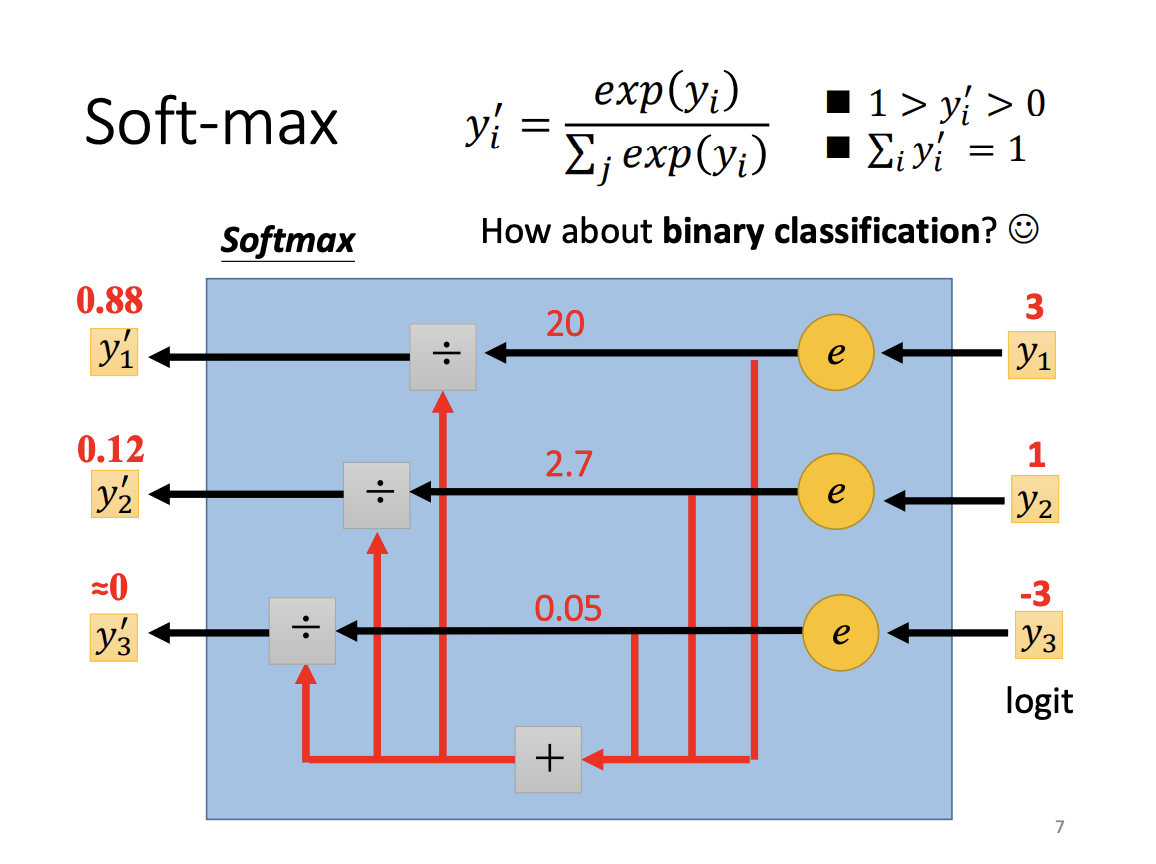
In practice, a softmax function is often applied before the classification output. The purpose of softmax is to normalize the output probabilities between 0 and 1, which typically improves model performance. The input to the softmax function, known as the logit, is transformed through a process that emphasizes differences between class scores. Beyond normalization, softmax also magnifies the relative distances between the original class scores. For binary classification, however, the sigmoid function is used instead of softmax. While they share similarities, sigmoid is more appropriate for two-class scenarios.

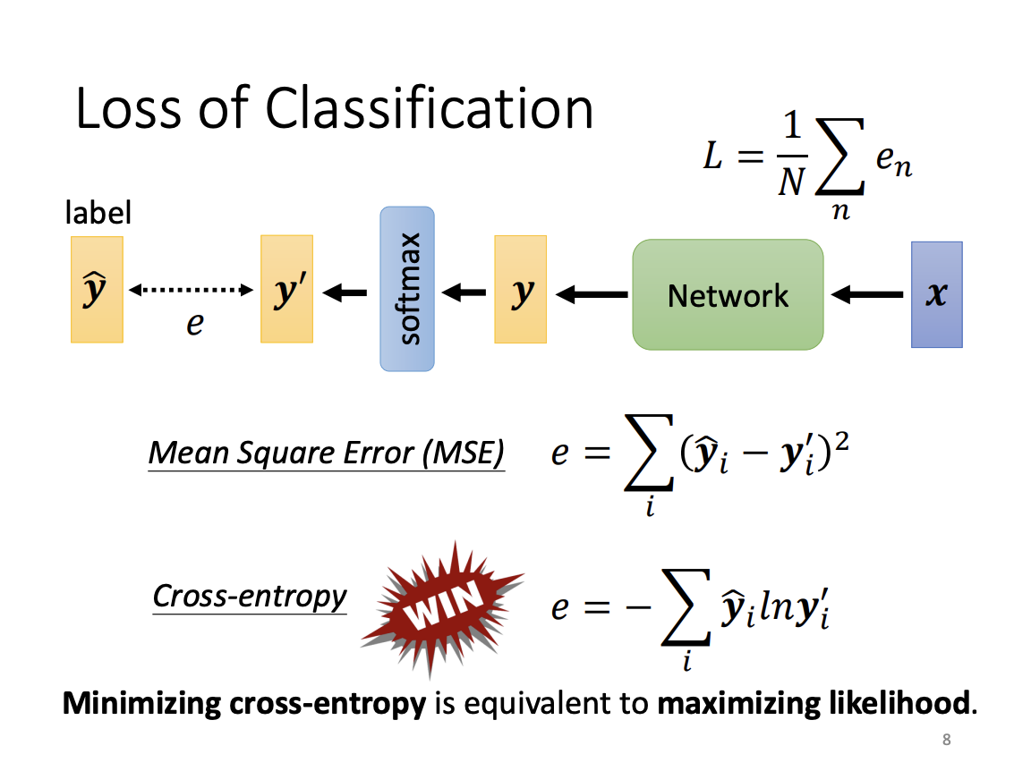
The loss function for classification measures the difference between the predicted output vector and the true label vector. Although mean squared error (MSE) can be used to compute classification loss, cross-entropy is preferred and more commonly employed. Minimizing cross-entropy is equivalent to maximizing the likelihood of the model’s predictions being correct.

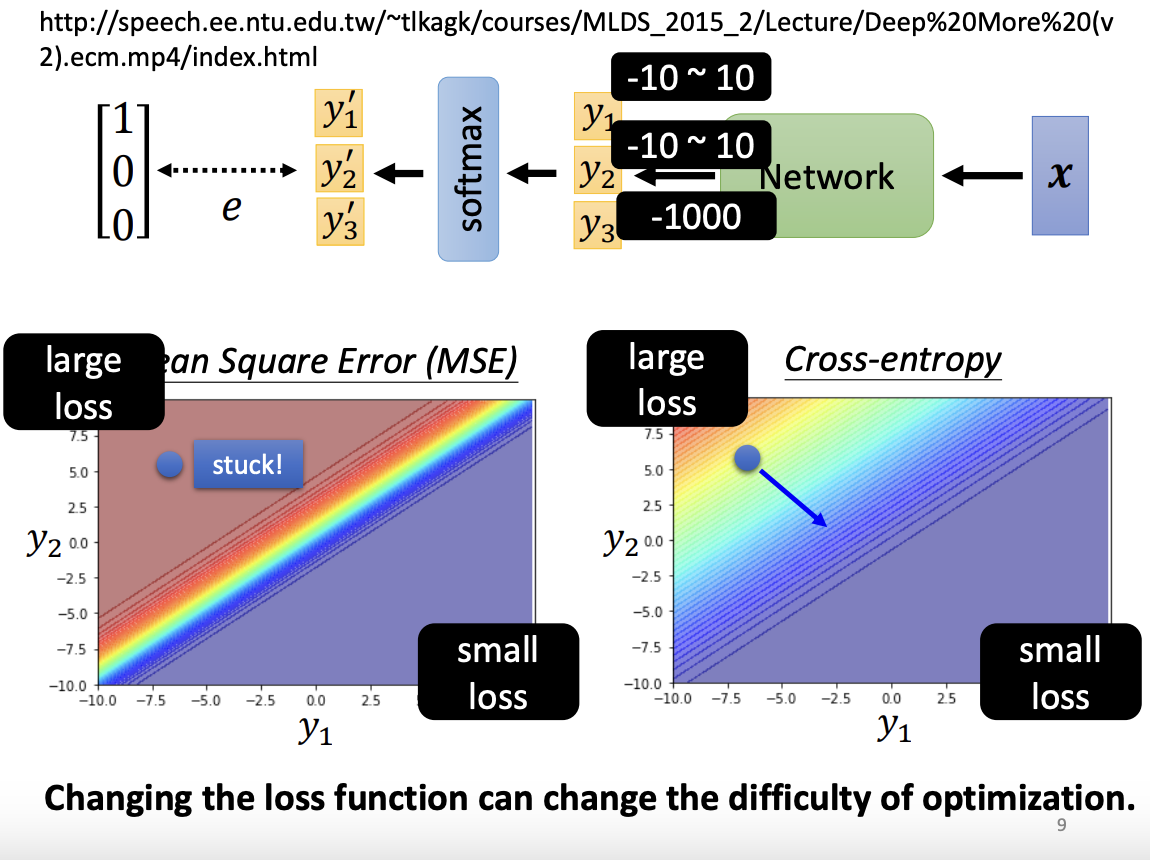
From a training perspective, cross-entropy often results in a smoother error surface compared to MSE, making it easier for optimization algorithms to converge to a lower loss. Thus, the choice of the loss function directly impacts the difficulty of the optimization process and the model’s ability to find optimal solutions.

Batch Normalization

While adaptive learning rates are designed to tackle difficult optimization surfaces, Batch Normalization can reshape the error surface itself, leading to more efficient training.

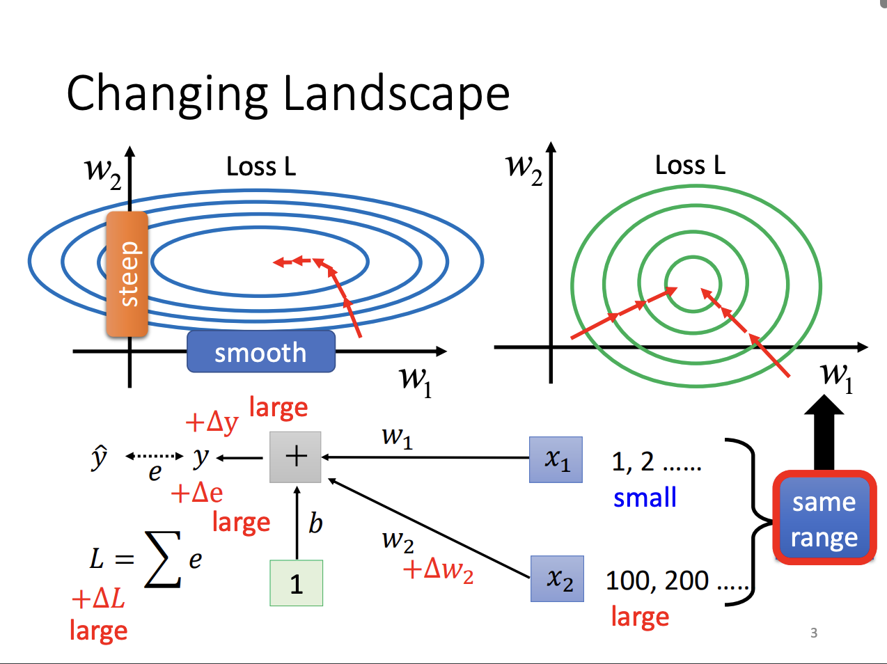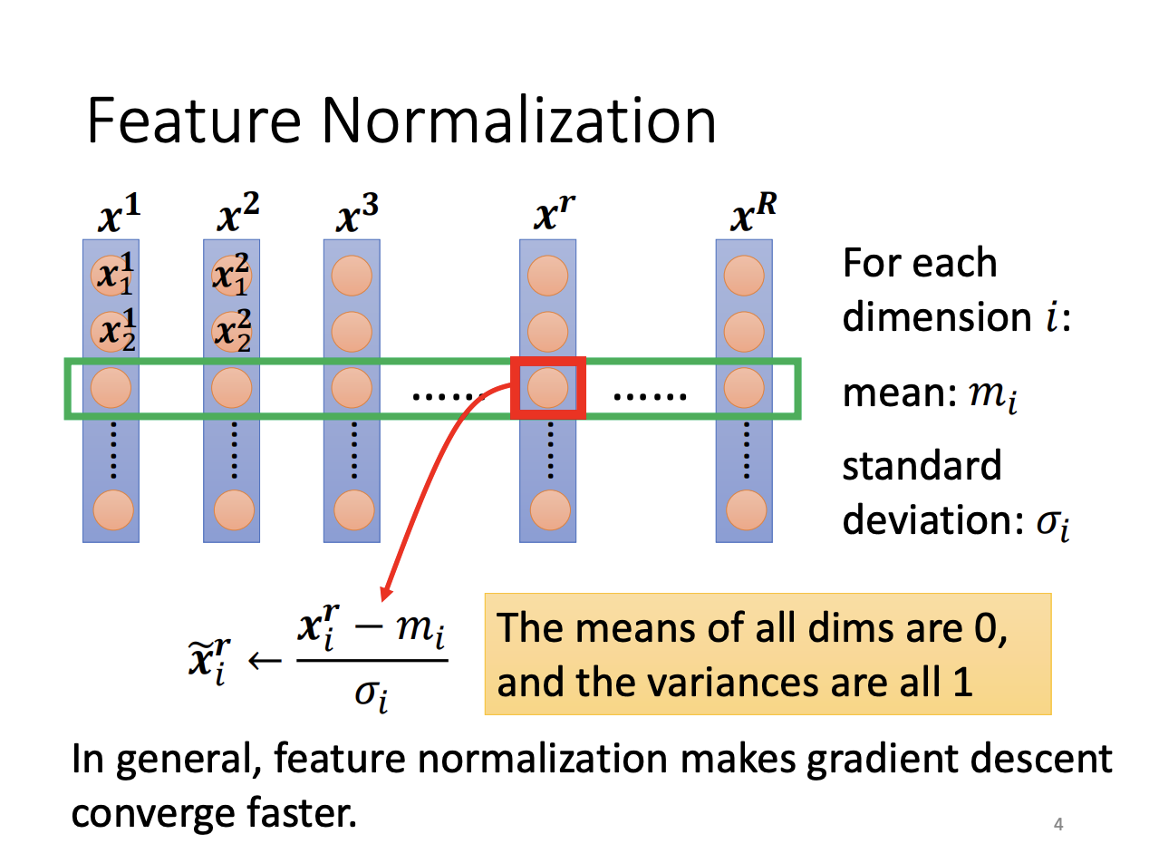
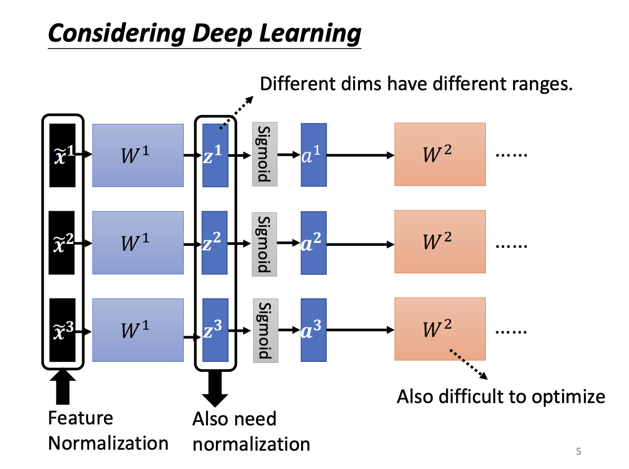
Feature normalization is a technique that scales different feature dimensions to similar ranges, making the error surface smoother and easier to navigate. In deep learning, normalization can be applied to each layer of the model. This normalization can be performed either before or after the activation function, although in practice, for functions like sigmoid, normalization is typically applied beforehand.

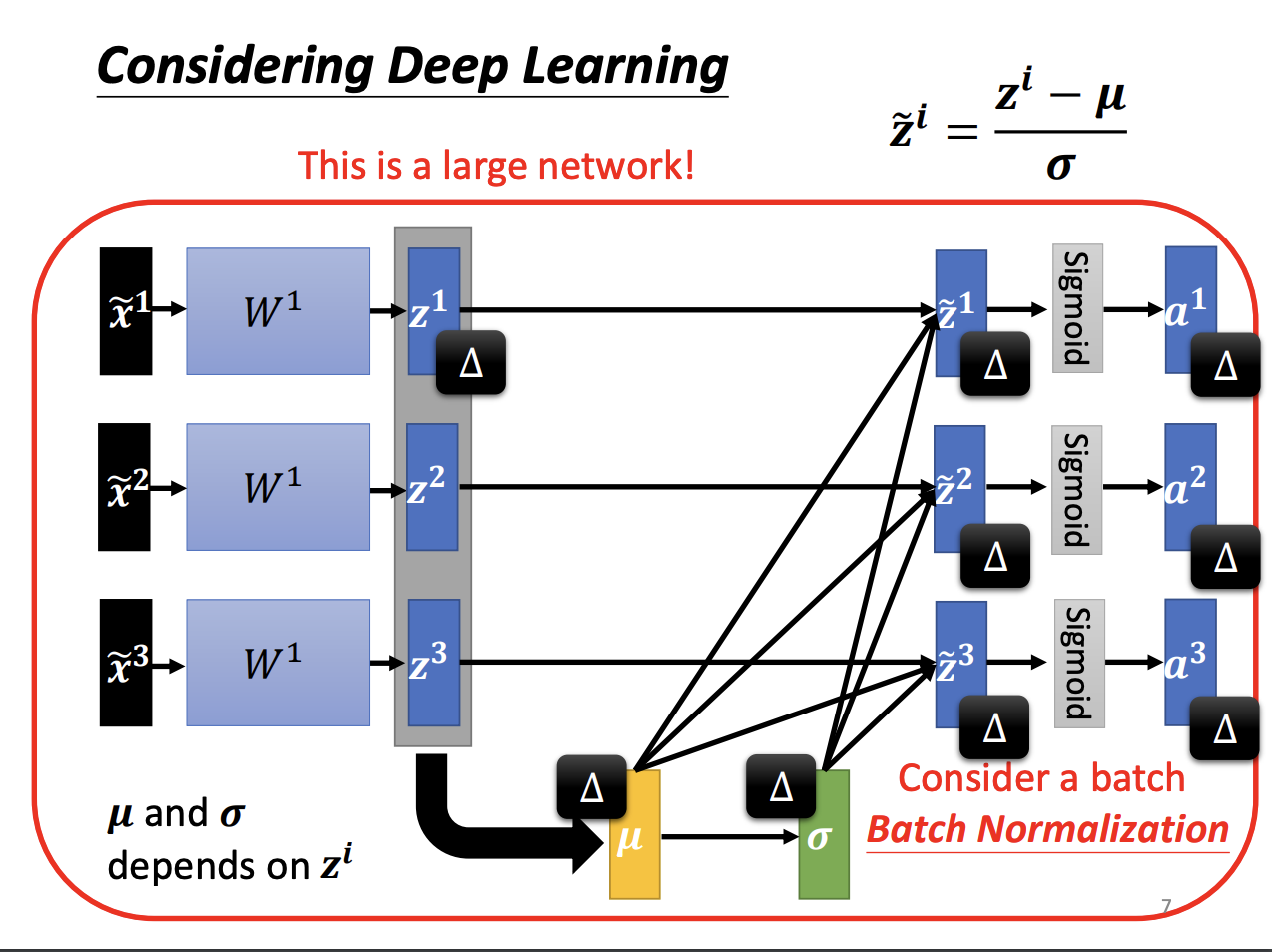
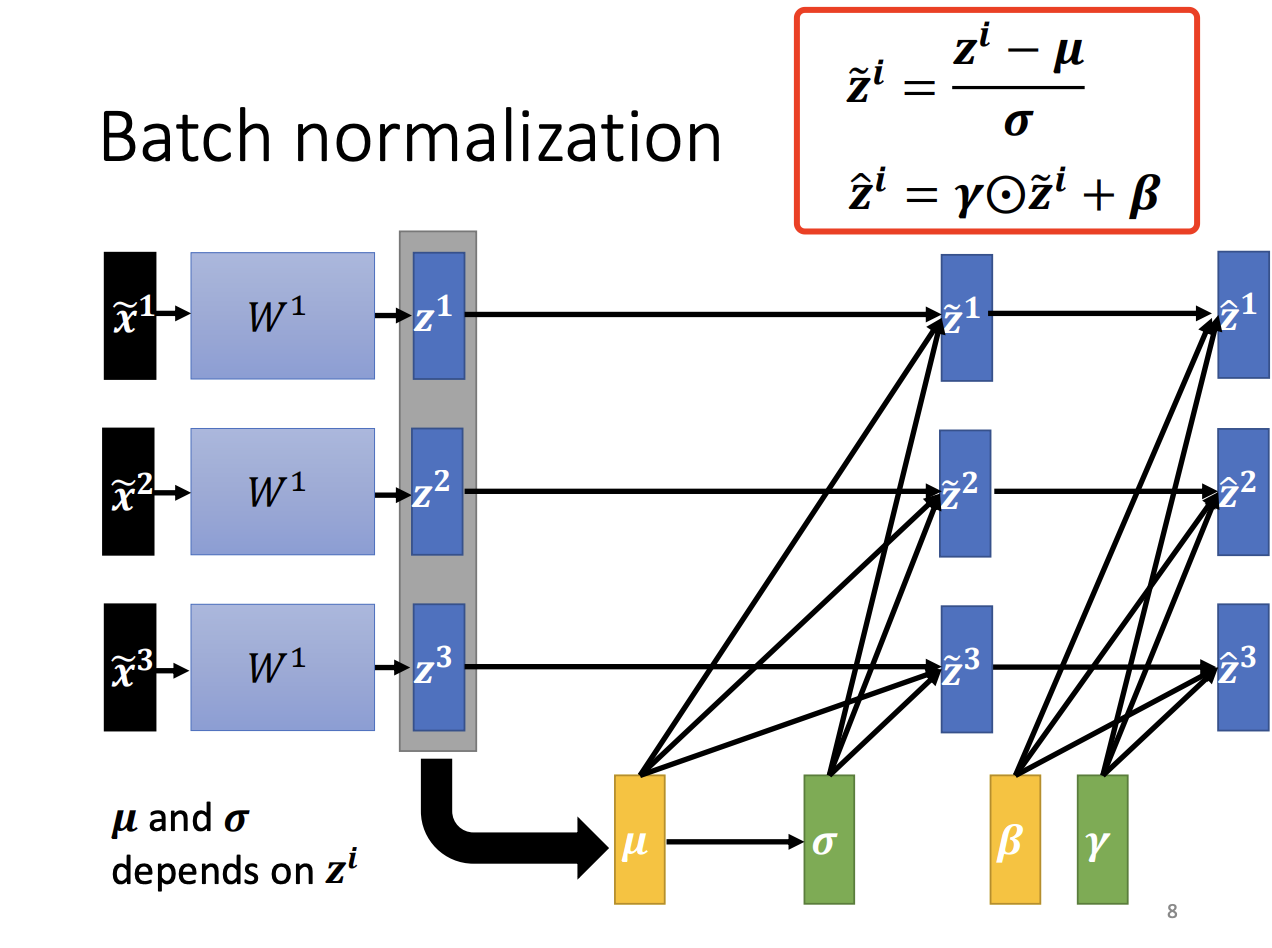
Batch Normalization is specifically named because the normalization parameters are computed based on each batch of data during training. The technique normalizes the activations within each batch to have zero mean and unit variance, which helps mitigate issues related to internal covariate shift.
However, concerns arise that strictly normalizing the activations to have zero mean might limit the expressiveness of the model. To address this, two additional parameters, gamma and beta, are introduced, allowing the model to maintain a non-zero mean and a more flexible scaling of the hidden layer outputs. These parameters are learned during training and allow Batch Normalization to adapt to the data distribution, further improving model performance.