[ML] Deep Learning

Machine Learning

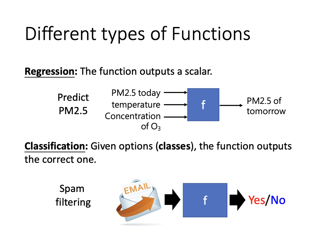
There are three primary objectives of machine learning, regression, classification and structured learning.

1. Basic concepts

• Model
  Model is constructed based on domain knowledge and is used to define the function that calculates result.
• Feature
  A feature represents the input to the model.
• Unknown Parameter
  An unknown parameter is a value in the model that remains to be calculated or learned from the data. In the model y = b + wx, b and w are the unknown parameters.
• Weight
  In model y = b + wx, w is referred to as the weight.
• Bias
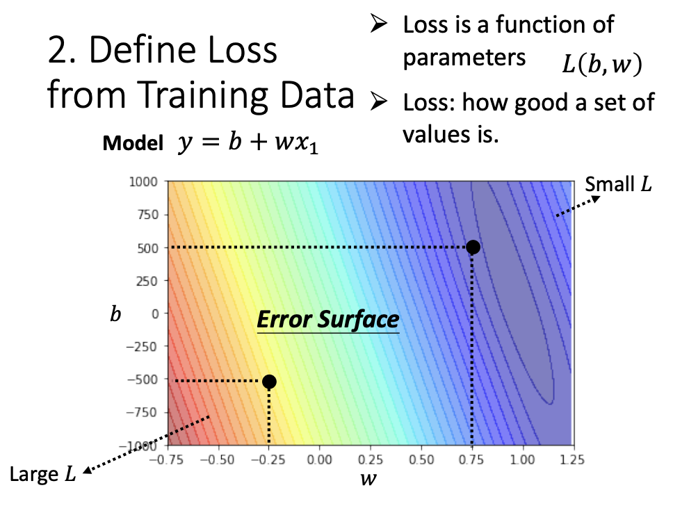
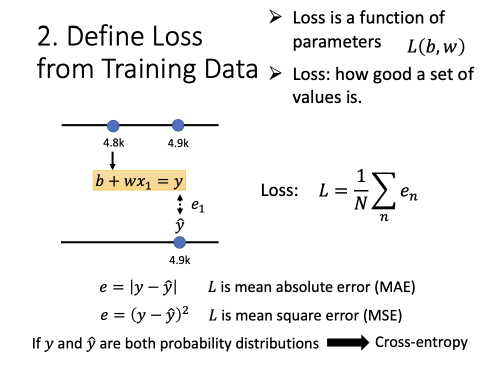
  In model y = b + wx, b is referred to as the bias.
• Loss
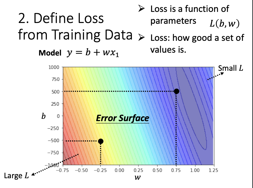
  Loss is function of parameters, denoted as L(b, w). It describes how well a set of values compares with the training data.
• Error Surface
  The error surface illustrates the relationship between loss and the unknown parameters, demonstrating how loss changes with different parameter values.

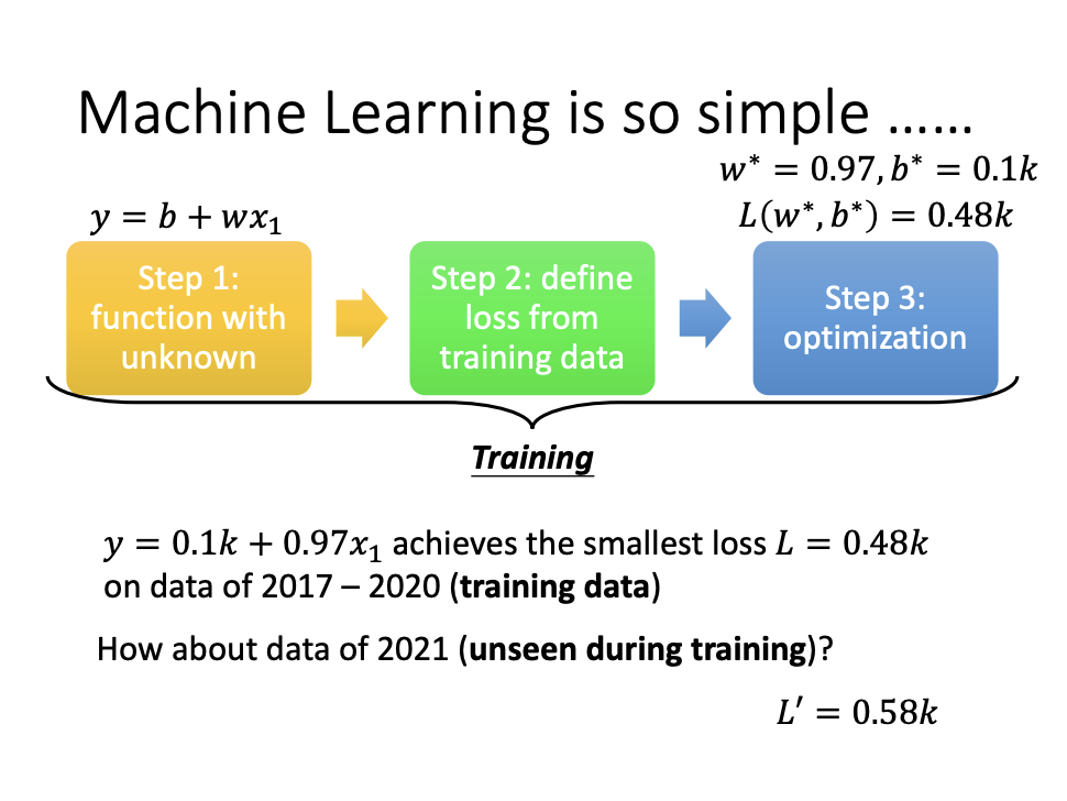
2. Procedure of Machine Learning

The machine learning process can be succinctly described in three steps, collectively known as training:

1. Guess a function with unknown parameters.
2. Define loss from training data.
3. Optimize the function to minimize the loss.

3. Model

Linear Model

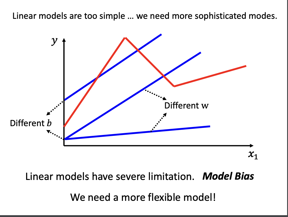
Designing a model involves creating a function with unknown parameters, and the linear model is the simplest form.

• $y = b + wx$
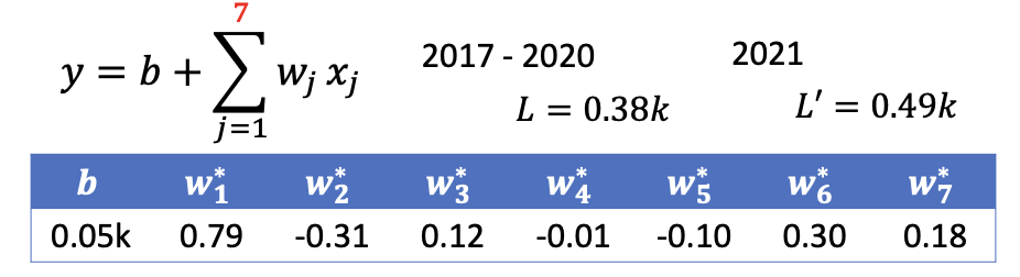
  to predict future base on a single past data point.
• $y = b + \sum_{j=1}^{7}w_jx_j$
  to predict future base on multiple past data points.

While linear models are straightforward, they may not accurately represent reality in all cases, as not all relationships are linear. The discrepancy between the model and reality is referred to as Model Bias

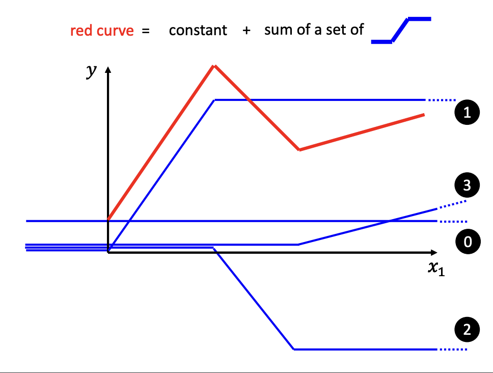
Piecewise Linear Curves

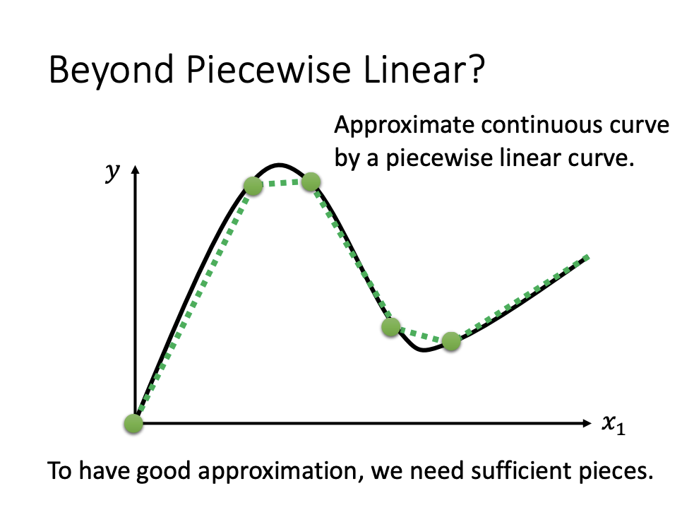
For more flexible modeling options, Piecewise linear curves are one alternative.

A piecewise linear curve is formed by combining multiple linear segments. This approach allows for the approximation of complex curves, as illustrated in the accompanying image.

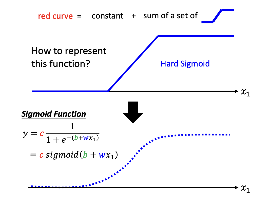
Sigmoid Function

Similar to linear functions, the sigmoid function can also approximate a curve (hard sigmoid).

• $y=c * sigmoid(b + w *x) $
  base on a single post data point, x.

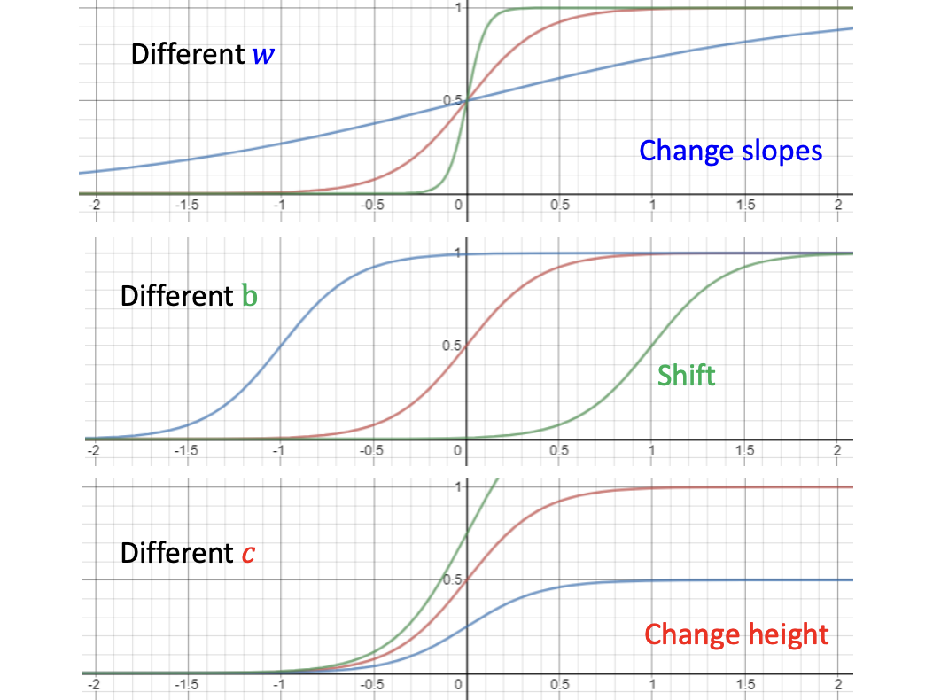
The function above describes how y changes based on a single past feature, x, using the sigmoid function. The curve can be adjusted by modifying the parameters w, b, c.

• w: controls slopes.
• b: shifts the curve.
• c: adjusts the height.

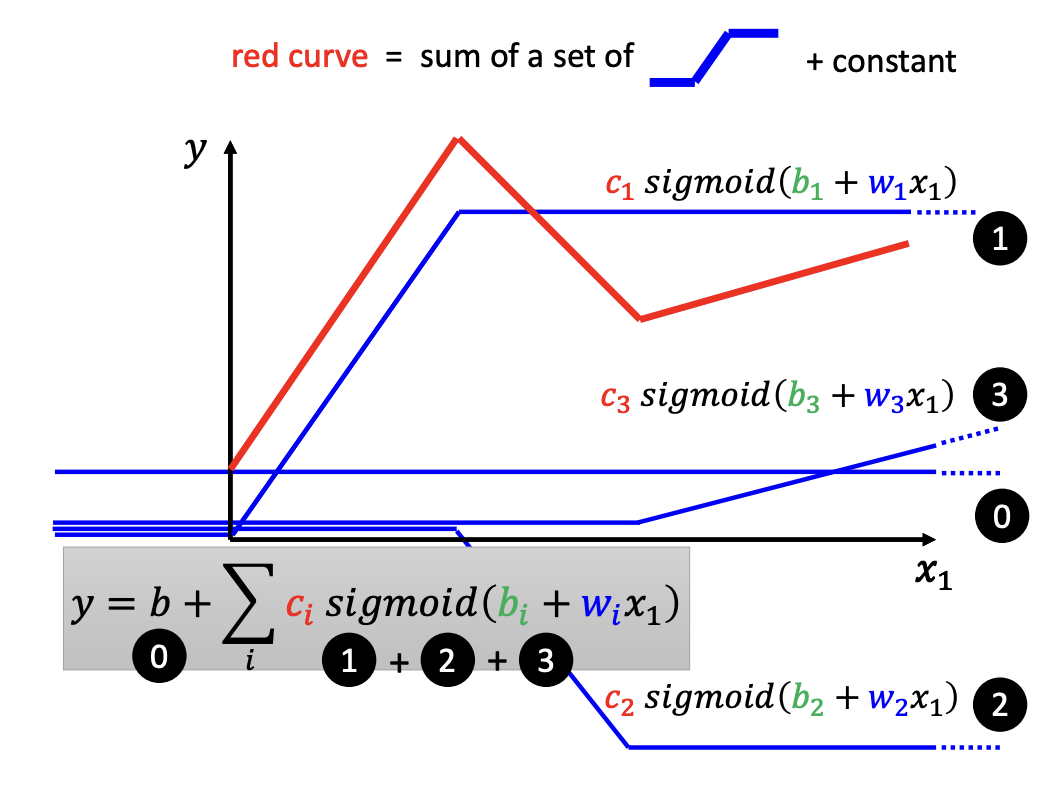
Like piecewise linear curves, multiple sigmoid functions can be combined to represent a complex curve:

• $y = b + \sum_{i}^{}c_i * sigmoid(b_i + w_i * x)$
  base on a single past feature, x.

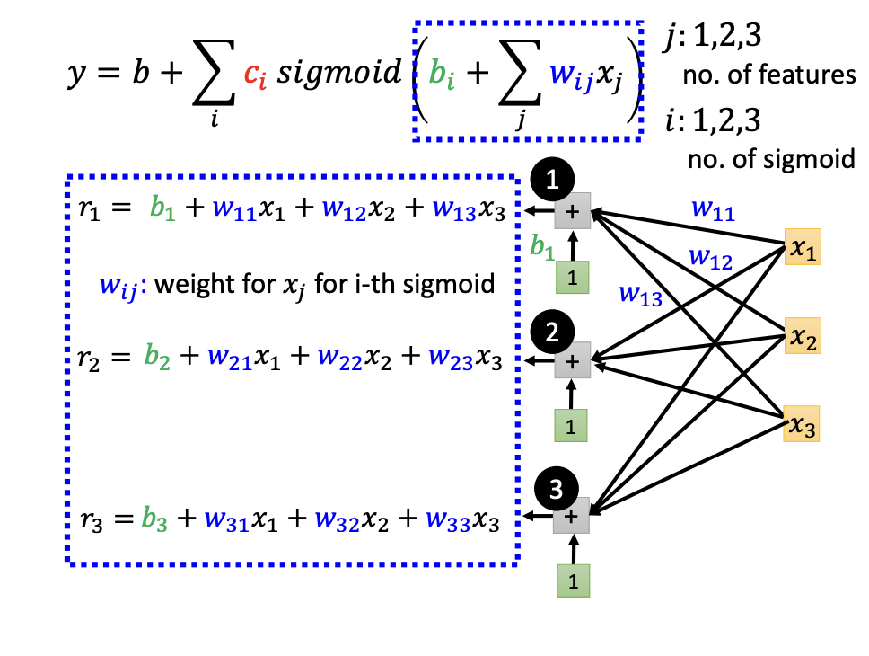
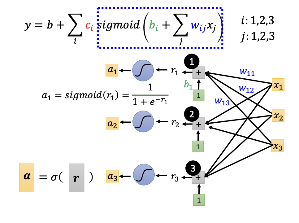
When considering multiple features, where y is calculated based on several x values, the sigmoid function can be expressed as:

• $y = b + \sum_{i}^{}c_i * sigmoid(b_i + \sum_{j}^{} w_{ij} * x_j)$
  base on multiple past features, x_j.
  i represents the number of sigmoid functions.
  j denotes the number of features or past data points.

Multi Sigmoid Function based on multiple Features

At first glance, the function above may seem complex, as it involves multiple sigmoid functions based on multiple features.

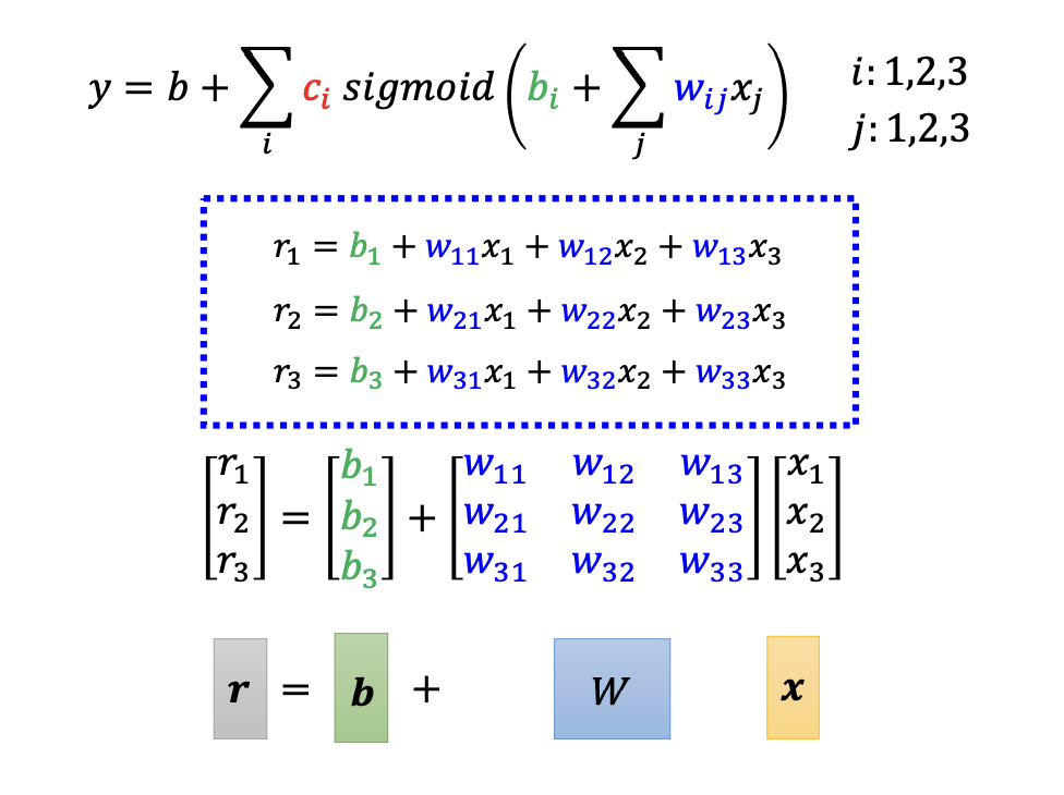
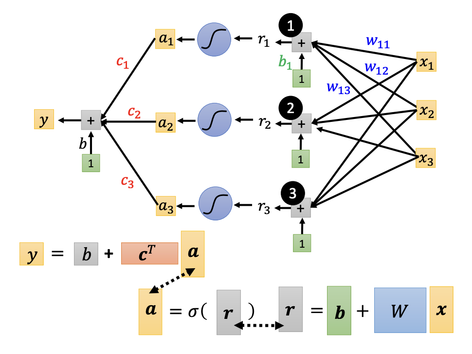
However, the expressions inside the sigmoid functions can be represented in matrix format, which simplifies understanding and computation.

• $r = b + W * x$
• $a = \sigma(r) $
• $y = b + c^T * a $

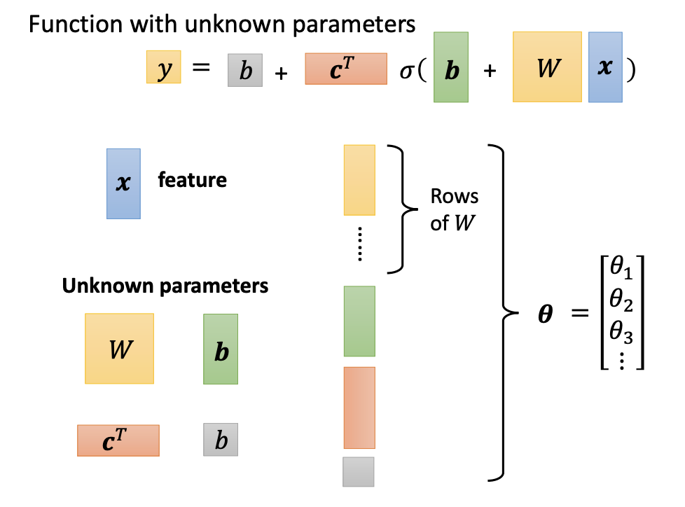
In matrix format, the function can be described as follows:

• $y = b + c^T * \sigma(\vec{b} + W * \vec{x}) $
  $\vec{x}$ represents the feature vector
  W, $\vec{b}$, $c^T$, b are unknown parameters
  all parameters can be consolidated into a single vector, denoted as $\theta$

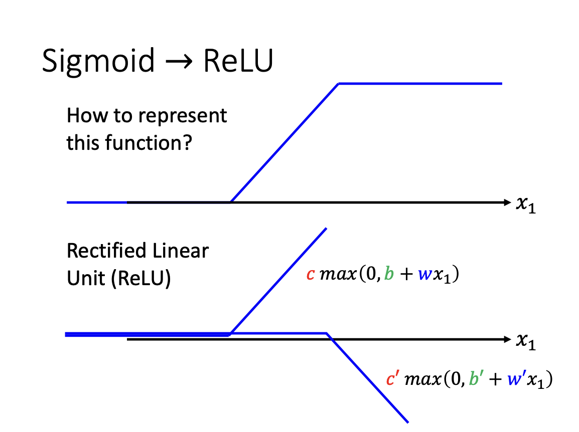
Activation Function

In addition to the sigmoid function, the ReLu(Rectified Linear Unit) is another function to build a model, which is often faster to compute.

• $y = c * max(0, b + w * x)$

Collectively, these functions are referred to as activation function.

4. Loss

Loss is a function of the parameters that quantifies the quality of a set of values. Two of the most common loss functions are Mean Absolute Error (MAE) and Mean Squared Error (MSE).

5. Optimization

Optimization involves adjusting the unknown parameters to minimize the loss. One common method for achieving this is Gradient Descent.

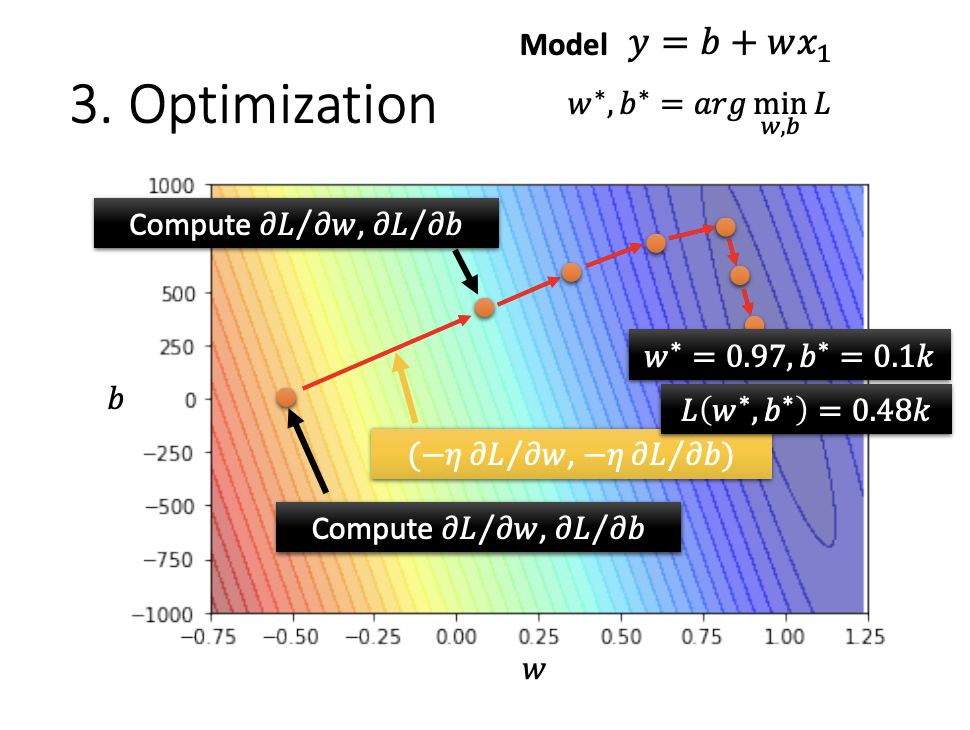Through gradient descent, we can determine how to adjust parameters to achieve better results. Ideally, after a certain number of iterations, we will identify the parameters that yield the lowest loss. However, in most cases, we will stop due to a predefined maximum number of iterations. If we set a maximum of 1,000 iterations, this value is referred to as a hyperparameter.

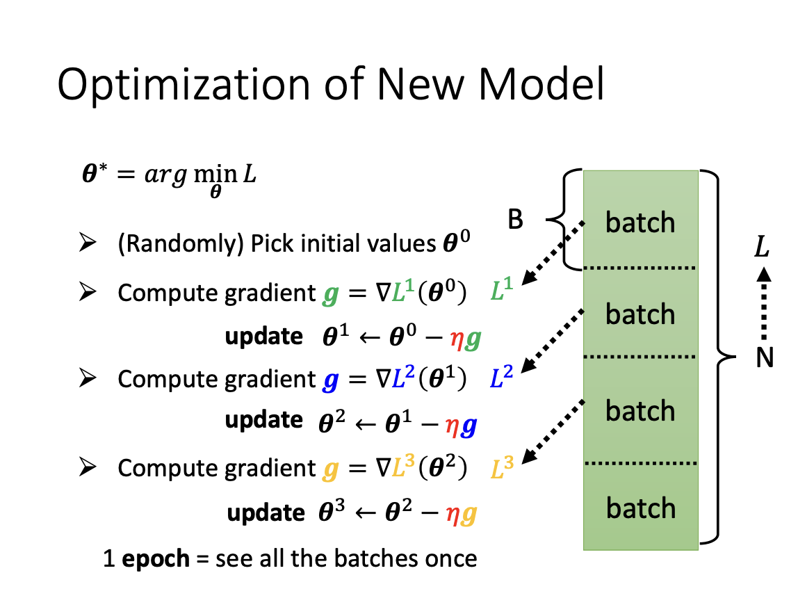
During the optimization of a model, a list of examples is used to adjust the parameters, typically processed in multiple iterations rather than all at once. In each iteration, a batch of examples is consumed, which is referred to as an update. Once all batches have been processed, it is termed an epoch.

6. Deep learning

Each individual activation function, such as a single sigmoid or ReLU, is referred to as a Neural. When multiple activation functions are used to approximate a complex curve, the collection of these neurons forms a Hidden Layer. By stacking multiple hidden layers, we create a structure known as a Neural Network. Since this architecture can have many layers, it is termed Deep Learning.